Search kind of sucks nowadays. Even a simple query likely yields pages of “slop” content that hijacks SEO in order to suck-in traffic and steal advertising dollars. The situation has gotten so bad, that people have resorted to appending site:reddit.com to their queries in order to try to more pertinent results.

For a while now, I have wondered, why is search so hard? In order to better understand the inner workings of search engines, and as a fun side project, I decided that it would be cool to try to build my own version of a search engine.

I wanted to see if modern AI-enhanced approaches could make the experience feel closer to how search should work. Instead of SEO trickery, what if a search engine could actually understand the meaning of your query, and return exactly what you are looking for?

Google back in 2010 was crazy. You could look up anything and it’d be there.

— Daniel (@growing_daniel) August 16, 2023

My Background with Search Engines

One of the core courses I had to take toward my CS is called CS50: Software Design and Implementation. The course is all about how to structure & document code, as well as how to work collaboratively using tools such as git. One of two culminating projects for this class was to build a “tiny search engine”, nicknamed TSE.

The whole build process included crawler, indexer, and querier modules with full scoring and ranking. The project was built in low-level C, which meant that we had to reimplement data structures such as hashtables, counters, and sets; fully manage memory allocation; and interface with system-level file and networking protocols.

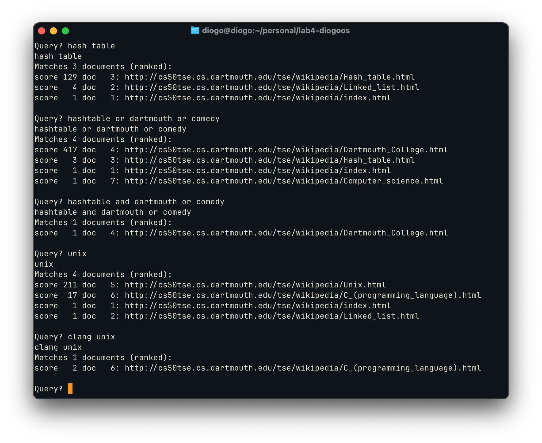
A demo of a TSE query running on my Linux on MacOS setup

Unfortunately, the code for TSE cannot be made public, at least while the CS curriculum remains the same (which it likely will for a very long time). However, for my new search engine project, I want to start from scratch again anyways. The original TSE only crawled a small clone of several wikipedia pages, had no semantic search, and used a rather rudimentary algorithm to score results.

Now, I want to focus less on the low-level aspects, and instead incorporate modern techniques. This means that we won’t be completely rewriting the file stack, and instead use modern technologies to augument search.

Embeddings: an overview

Vector embeddings are a way of representing text as points in a high-dimensional space. Instead of thinking of words as discrete symbols, we map them into numerical vectors (usually 384-dimensional or 768-dimensional real-valued arrays) such that semantically similar words or sentences end up close together.

The advantage of using embeddings is that they are able to capture deeper relational meaning between words that other techinques, such as one-hot enconding, are not. For example, the difference between the vectors for man and woman points in roughly the same direction as the difference between king and queen. ¹

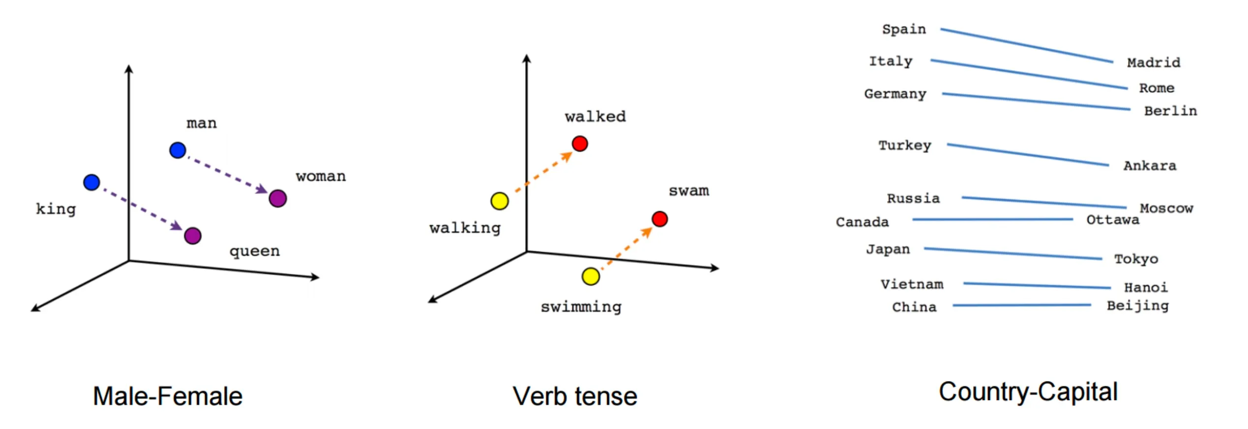
In the context of search, we extend this concept to sentences, allowing us to perform semantic search: instead of matching keywords, we can measure geometric proximity in vector space, and retrieve the text that is closest in meaning.

One of the most well-known embedding models is BERT, created by Google Research. BERT introduced the idea of pretraining a tranformer model using by a masked language modeling objective (like a fill-in-the-blank), and fine-tuning it for downstream tasks. The embeddings produced by BERT capture bidirectional context, meaning they encode information from both the left and right of a given token, which leads to much richer semantic representations than earlier methods.²

Building on this, more recent work has explored contrastive learning as a way to create high-quality sentence representations for fine-tuning models. Given pairs of semantically similar texts, the model is trained to bring their embeddings closer together, while pushing apart embeddings of unrelated sentences. This has become the standard approach for fine-tuning models for semantic search and retrieval tasks.³

Proof of concept: Wikipedia embeddings

To validate the approach, I built a simple proof of concept using vector embeddings for semantic search. Mirroring the TSE project, I first chose to index a set of Wikipedia pages, as the index is relatively small & has mostly useful information. However, instead of mirroring the full database (whose full contents are >1TB decompressed), I used the Simple English Wikipedia, which is only ~365MB and contains shorter sentences, reducing both storage and embedding time.

I chose to build initial proof of concept in a Jupyter notebook. Using the wikitextparser package, I filtered out all the MediaWiki syntax, links, and more, returning clean (title, url, text) tuples. I then used NLTK to tokenize each article’s content sentence-by-sentence, so that retrieval could be done at the sentence level rather than only at the page level.

For embeddings I began with a pre-trained model to create the vector embeddings, namely all-MiniLM-L6-v2 provided by the sentence-transformers package. This model outputs 384-dimensional vectors designed for semantic similarity tasks. Since the purpose of this initial test was just to showcase the relative performance of using vector embeddings, this did exactly what I needed.

As an important aside, processing all this data in a single thread would take a very long time. So, for both the plain text parsing, as well as for the creation of embeddings, I made use of a producer-consumer paradigm (thanks CS 10!) to speed up the process, as follows:

I include this code here mostly as a reference for future projects: I am not very familiar with Python built-ins like ThreadPoolExecutor, so this template is super useful for use in future compute-intensive tasks.

Once the indexing was completed, we were able to evaluate a sampling of the results when using these methods:

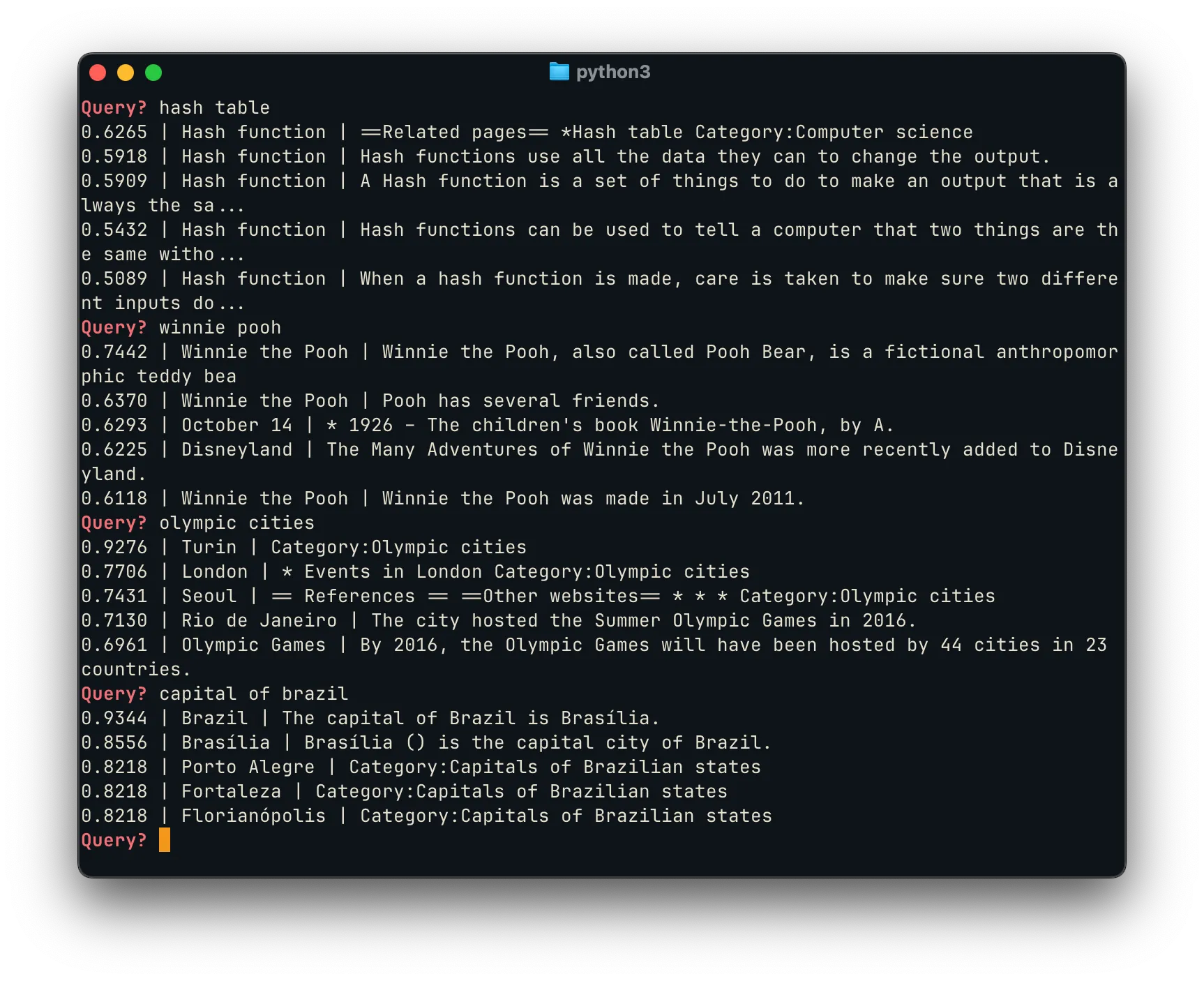The top results for each query proved to be highly relevant, with scores reflecting strong semantic matches. For example, “capital of brazil” correctly surfaces Brasília as the top result, and shows the capital of other Brazilian states as highly-relevant alternatives. Likewise, a query for “olympic cities” returns cities that have hosted the Olympics, as well as a page generally linking to the “Olympic Games” directly.

An interesting feature of using a sentence embedding database, rather than just a word-based index, is that the model can point you to the direct answer to a query. This works well for the retrieval of factual information of various kinds:

Q: quentin tarantino style
Quentin Tarantino’s filmmaking style is characterized by non-linear narratives, sharp dialogue, pop culture homage, strong female characters, graphic violence, eclectic soundtracks, masterful pacing, playful narrative references, lush visuals, and narrative closure.

Q: latest us president
The current President of the United States is Donald J Trump.

Q: highest mountain USA
The highest mountain in North America is Mount McKinley (6,194m) in Alaska.

The latter two of these examples really help to highlight the value of embeddings, where simple text-based searches might otherwise fail. The cosine distance between latest and current is small, allowing us to surface the correct information about the president, even when the query is phrased slightly differently. Similarly, the last example response does not match the ‘USA’ keyword exactly; however, the terms North America and Alaska are encoded as vectors close to USA, allowing the answer to be surfaced nonetheless, as if the underlying system “understands” our requests.

Simple Wikipedia Search Tool

Satisfied with the general performance of this basic model, my next step in this project was to build a better Simple Wikipedia Search Tool that performed well, but was somewhat more robust and efficient. This tool had to address three main problems with the proof of concept:

1. While we were previously storing embeddings in a simple jsonl file, this was very storage & memory inefficient: we had to load all the embeddings & all the metadata at once, then query into it. This led to a substantial performance hit, as it took several minutes to load everything into memory, and led to the Python process taking up ~10GB of memory.

2. Chunking input into sentences was useful, but the sentences were too small and often led to a loss of context. For example, when we indexed the sentence: “It was the first of its kind.”, without the previous paragraph pointing out what it is, the embedding is too broad and isn’t useful for search.

3. Since the vector search was across chunks, the same page would show up on the results overview multiple times. Instead of having repeated results, since we are emulating a search engine, it would be preferable to instead rank these pages higher, as they are more relevant, and show other pertient options below it. It would also be better to have a minimum score cutoff, to prevent irrelevant results from polluting the search when no/few good matches were found.

Memory Efficiency & FAISS

Firstly, to solve the memory efficiency problem, I made use of the faiss package from Facebook Research, which is designed for fast similarity search on large vector datasets. Now, instead of keeping all embeddings in Python memory as numpy arrays, FAISS stores them in an optimized index structure on disk, enabling very fast searches.

In addition to FAISS, we need to keep a metadata file containing the information needed to reconstruct the search results once FAISS returns a match. Thus, for each chunk, we also store a unique ID that corresponds to the embedding in the FAISS index; the URL of the original Wikipedia page the chunk came from; and text of the chunk itself, so we can display it in search results or pass it to downstream processing.

Using this method, we can query millions of embeddings much faster, and without having to load all the embeddings or all the chunks. Since the IDs assigned by FAISS are sequential, we can store hte metadata in a jsonl file, where each line corresponds to metadata for a given entry. Thus, we can lazy-load only the metadata needed for the retrieved entries.

These optimizations reduce the process footprint from 10GB to a fraction of that. Moreover, since the storage of the embeddings is also much more efficient, the total storage footprint of the search tool was reduced from ~6.5GB to only 884MB, of which 742MB is FAISS index, and 142MB is the gzip’d metadata. In total, that’s an almost 6x reduction in storage.

Chunking and ranking

To solve the second issue, I moved from sentence-level chunks to 200-word chunks with a 50-word overlap. This more balanced approach keeps enough context for the embeddings to make sense, while still keeping the text segments manageable enough for the vector model. Having the overlap ensures that content at the edges of chunks isn’t lost and allows, the embeddings to retain connections across sentences and paragraphs, solving the previous issues.

Finally, to prevent duplicate page results, the search tool now groups result by the original page and ranks pages by the highest scoring chunk. If multiple chunks from the same page match the query, we only show the page once at the top with the highest score, while other relevant pages appear below. Additionally, we manually increase the score of pages with multiple chunks, since having everal high-scoring chunks from the same page is a strong signal of relevance. Lastly, a minimum similarity score cutoff filters out poor matches, ensuring that only genuinely relevant pages appear in the results.

Results

In practice, the search tool consistently surfaces informative and relevant content for a wide variety of queries. The results show a natural ranking of importance, highlighting the most pertinent pages first while still offering additional context from related content. Overall, the outputs feel relatively organized and coherent, giving users meaningful answers without overwhelming them with noise.

• 
• 
• 

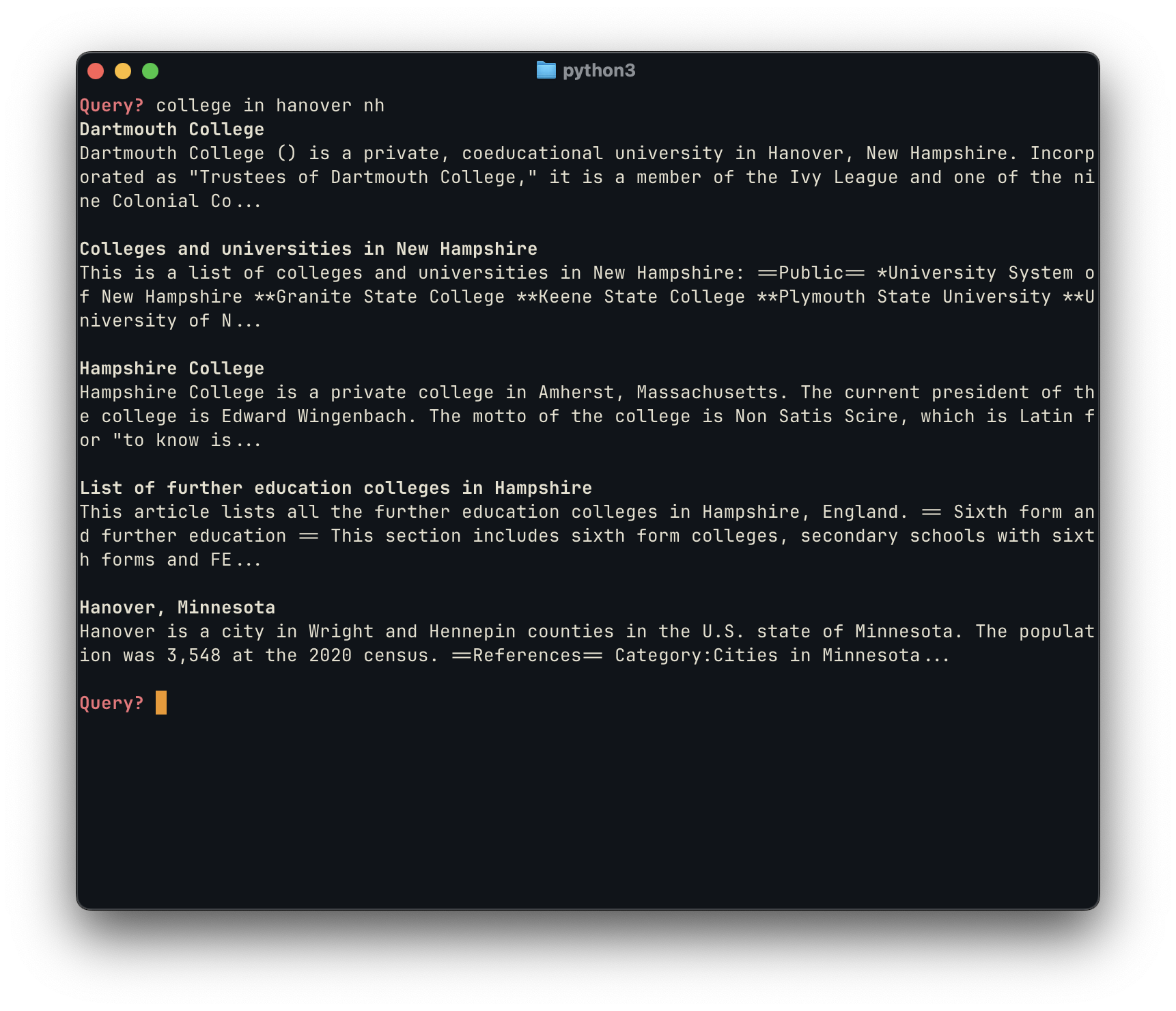
The examples above, similarly to the initial proof of concept, are particularly good because they are able to find the “intent” behind these queries, highlighting the semantic similarity between “NH” and “New Hampshire”, for example, and surfacing relevant content.

AI-augmentation

So far, the process of building this search engine hasn’t really involved much of the ‘AI-augmentation’ the title of this post had previously promised, beyond the use of embeddings. But those don’t really count as AI in the sense most people expect:

“[Embeddings] are foundational for artificial intelligence (AI). Technically, embeddings are vectors created by machine learning models for the purpose of capturing meaningful data” - Cloudflare

So, really, all we have done is use fancy statistic models — which is not quite what you’d pitch as a VC-backed B2C AI-powered SaaS digital platform. So, where can we use AI to improve this process?

1. Query optimization

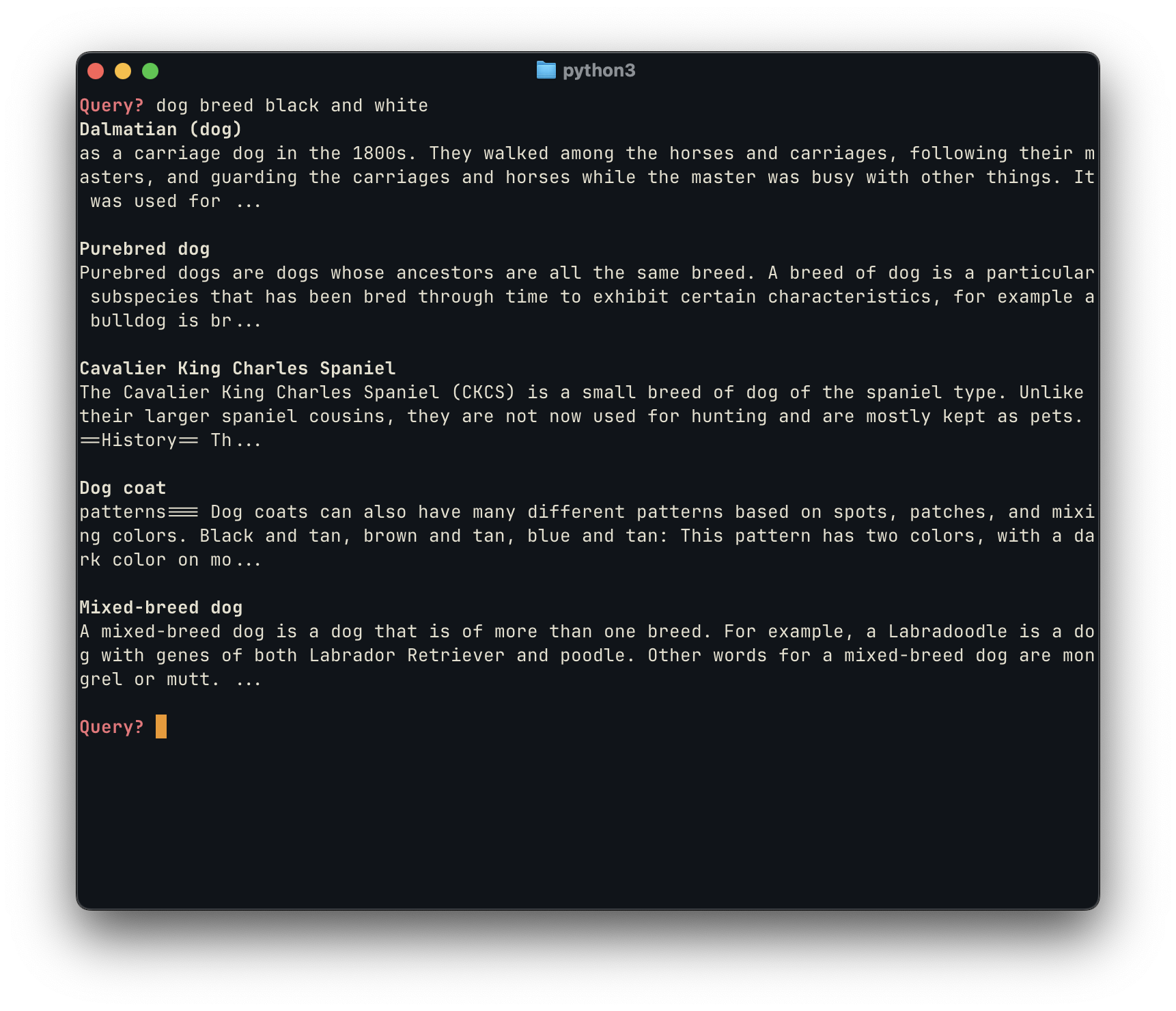
Users rarely type queries in the most “search-friendly” way. A simple example: someone searching “dog breed black and white” probably means “list of dog breeds with black-and-white coats.” An LLM can act as a query rewriter, transforming short, ambiguous user inputs into clearer, semantically richer queries. This makes the search more accurate and helps retrieve results that are closer to what the user actually wants, not just what they typed.

2. Cross-ranking

Our current ranking relies mostly on embedding similarity. That works, but it doesn’t capture all the nuance. A lightweight AI model (or even a fine-tuned LLM) could serve as a cross-ranker: once we’ve got a handful of top candidate results, the model re-scores them by considering things like semantic closeness, diversity, or user intent. This mimics what modern search engines already do — a two-stage retrieval process where fast vector search narrows the field, and then smarter models refine the order.

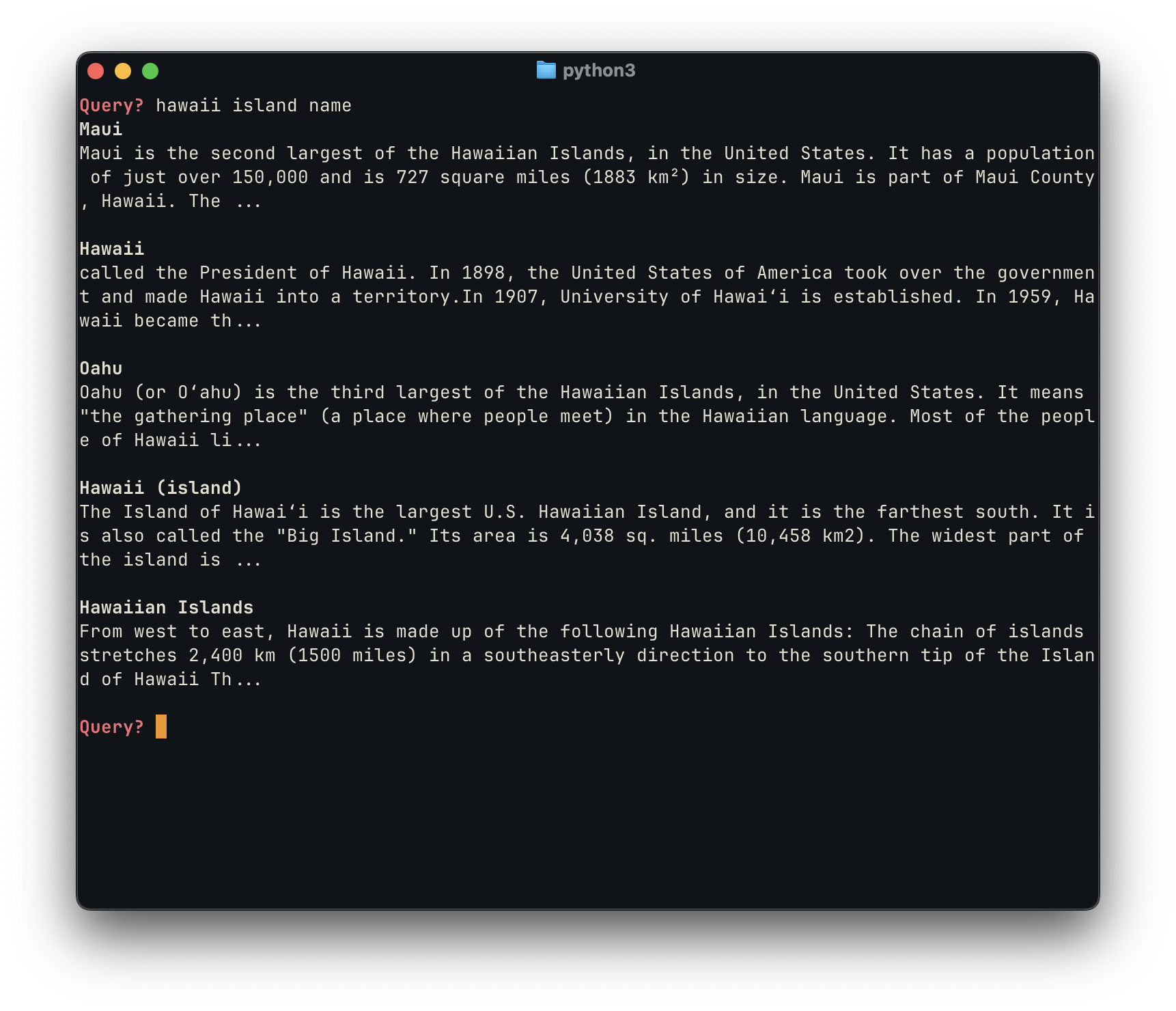
3. Retrieval-augmented generation

Finally, an LLM can sit on top as a summarizer, pulling together the key information from multiple chunks into a single coherent answer. Instead of showing five different Wikipedia excerpts about Hawaii’s islands, the tool could generate a concise, natural-language explanation: “Hawaii consists of eight main islands, including Maui, Oahu, and the Island of Hawai‘i…” This makes the tool feel less like a search engine and more like an assistant.

Moreover, by feeding the LLM some of the top-ranking embedding chunks, we can ground its summaries in factual context rather than letting it “hallucinate.” This approach, often called retrieval-augmented generation (RAG), ensures that the model has real source material to draw from. The LLM doesn’t have to invent answers, as it can extract and rephrase the relevant details from the retrieved passages.

Even better, because those chunks come with metadata (like the original page URL), the LLM can cite its sources alongside the generated summary. This not only increases trustworthiness, but also makes the results feel more like a search engine + AI assistant hybrid: concise, readable summaries with transparent references to where the information came from.

Building an AI-augmented (Wikipedia) Search Engine

Implementing these AI-powered optimizations to our existing model can be done pretty easily, by making use of existing pre-trained models and simply adding them to the querying chain. Since one of the driving ideas behind this project is that it should be locally-run (from creating the embeddings to processing queries), I refrained from using the OpenAI API and similar options, and instead used ollama to get an LLM model running locally. Even better results can be achieved by using one of these leading APIs instead.

Implementing query optimization

The first change I tackled related to query optimization, as it was one of the main drawbacks of the current model. Currently, we struggle a lot with compound queries: users might type things like “history or culture of Hawaii”, which might not cleanly match to the most relevant embeddings. This is where we can use an LLM as a query rewriter, expanding a short or ambiguous query into several semantically optimized alternatives. Here’s the system prompt that I came up to test this model:

You are helping optimize search queries for a semantic search engine.
Given a user's query, generate several alternative phrasings that
capture the different possible interpretations of the intent.  

- Expand short or vague queries into more descriptive ones.  
- Include options that use synonyms or rewording.  
- If the query seems to involve an "or" condition (two alternative ideas),  
  produce separate queries for each alternative as well as one combined
  form.  

Example 1: Simple query
User query: "dog breed black and white"
Example output queries:
	1. "List of dog breeds that have black and white coats"
	2. "Dog breeds with spotted black and white fur"
	3. "Examples of black-and-white colored dogs"
	4. "Dalmatian and other black-and-white dog breeds"

Example 2: Compound query
User query: "history OR culture of Hawaii"
Output queries:
	1. "History of Hawaii"
	2. "Cultural traditions of Hawaii"
	3. "History and culture of Hawaii"
	4. "Historical events that shaped Hawaiian culture"
	5. "Overview of Hawaii's history and cultural heritage"

Return the outputs in JSON form.  
For example: ["History of Hawaii", "Cultural traditions of Hawaii", "History and culture of Hawaii"].  

You must output only a JSON array containing only strings.  
Do not include any other text, explanation, or formatting.

An initial test with this system prompt showed very promising results. For example, for a test query of "budget airlines europe asia", the model was correctly able to identify and expand the compound query and generate a list of intents that would generate higher ranking results:

[
  "Affordable flights available in Europe or Asia",
  "Budget airlines operating in Europe",
  "Budget airlines operating in Asia",
  "Low-cost airlines in Europe and Asia",
]

Here, you can compare the performance of the search engine with and without this LLM query generation:

• 
• 

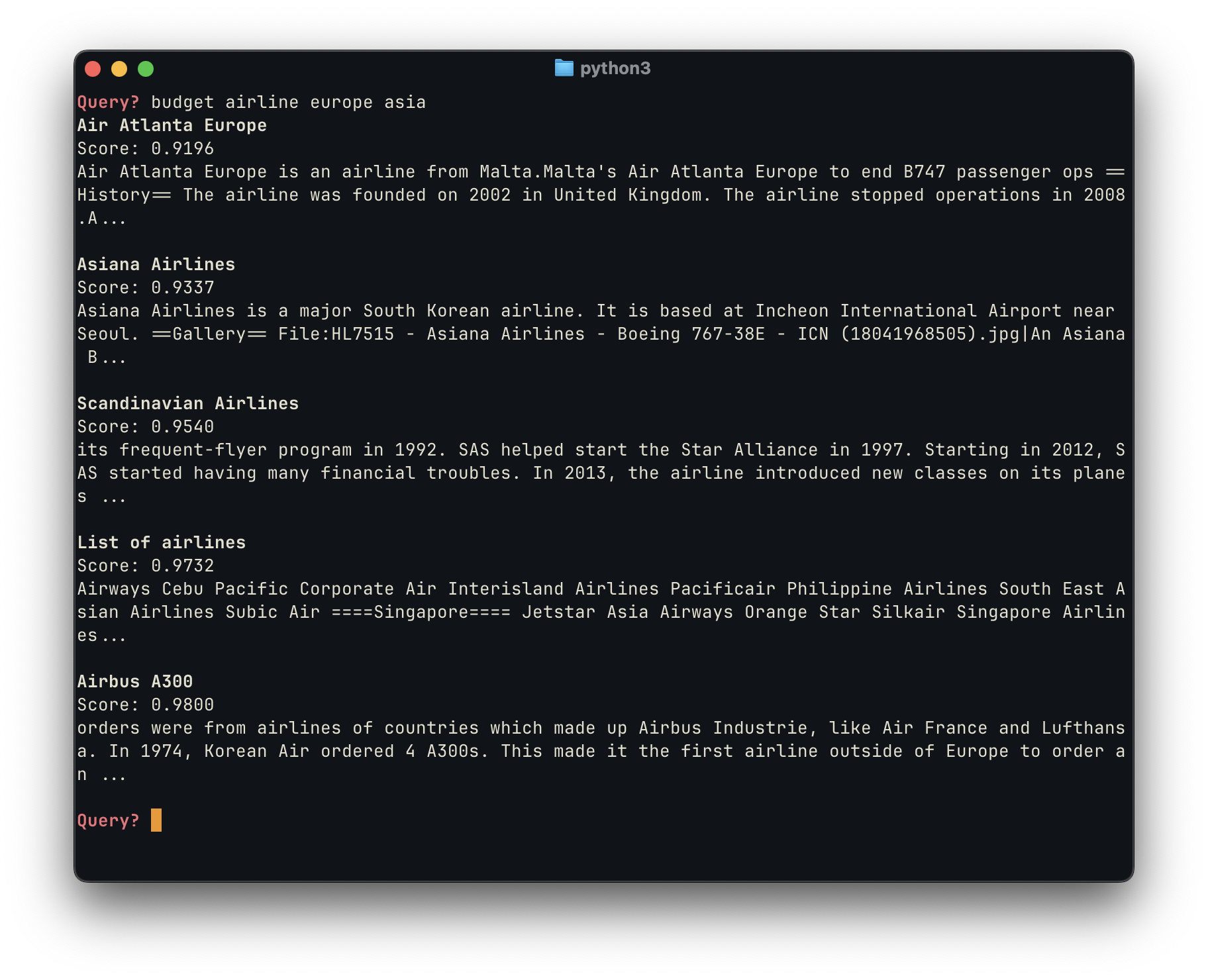
In the unoptimized search, we obtain a mixed bag of results. We first surface Air Atlanta Europe, which was a low-cost carrier, but is now defunct. Next, we do find one European and one Asian budget airline, which aligns with the user’s intent. However, the next results are very poor: they include a List of Airlines, which is too broad for this query; and it surfaces an article about the Airbus A300 which deviates from the user’s intent.

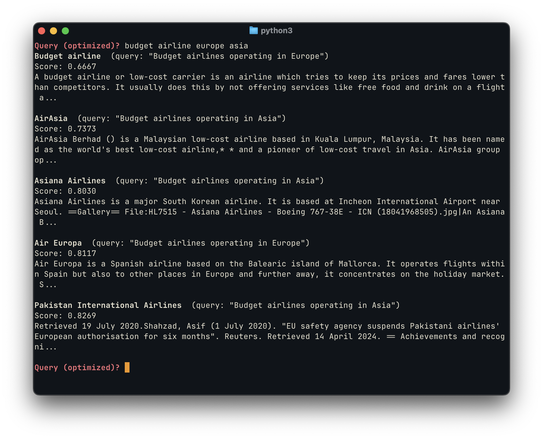
In comparison, by using the LLM-generated queries, we were able to obtain subjectively better results, with all five links directly pertaining to the the user’s query and intent. We first surface a broad overview article about budget airlines in general, which itself includes a list of airlines — then we include 4 low cost airlines that attend to the user’s intent, AirAsia, Asiana Airlines, Air Europa and Pakistan Airlines.

The power of LLM augmentation is objectively reflected in the much lower scores for each model. The unoptimized query ranges from 0.91 to 0.98, while the optimized ones are significantly lower, ranging from 0.67 to 0.82. (Note that, in this case, a lower score means semantically closer results, and thus is better.) This happens because two of the LLM-generated alternative queries, “Budget airlines operating in Europe” and “Budget airlines operating in Asia” are much closer semantic matches than other options — they perform much better the original query, as well as the other LLM-generated queries, and thus surface better results.

Implementing cross-ranking & snippets

Using the same LLM technique, we can cross-rank an even broader range of results, from across all the different query variations. I opted to again use a local LLM model, with the following prompt:

You are a search ranking assistant. 
Your task is to re-rank a list of candidate passages for a given user query. 
Rank the passages by how well they answer the query, considering both relevance and usefulness. 
Return a JSON object with each passage ID and a relevance score between 0 (not relevant) and 5 (perfect match).

Query: "{user_query}"

Candidate passages:
1. [ID: p1] "{passage_1}"
2. [ID: p2] "{passage_2}"
3. [ID: p3] "{passage_3}"
...
N. [ID: pN] "{passage_N}"

Output strictly in JSON format as:
{
  "p1": score,
  "p2": score,
  "p3": score,
  ...
}

I decided to use a weighted linear combination for the re-ranking of the results, with an adjusted weight between the retriever and LLM scores, normalized between 0 and 1. Some pseudo code for this process is shown below:

# Example scores
vector_distances = [0.72, 0.85, 0.64, 0.58]   # Euclidean distance
llm_scores       = [4, 5, 2, 1]               # LLM output (0–5)

# Convert distance to similarity
vector_scores = [1 / (1 + distance) for distance in vector_distances]

# Convert to numpy
vector_scores = np.array(vector_scores).reshape(-1, 1)
llm_scores = np.array(llm_scores).reshape(-1, 1)

# Normalize each to [0, 1]
scaler = MinMaxScaler()
vector_norm = scaler.fit_transform(vector_scores).flatten()
llm_norm = scaler.fit_transform(llm_scores).flatten()

# Combine with weighted sum
alpha = 0.6  # weight for retriever
beta = 0.4   # weight for LLM
final_scores = alpha * vector_norm + beta * llm_norm

ranking = np.argsort(-final_scores)  # descending order

Finally, the implementation of RAG follows a very similar approach, were a LLM model is given a general prompt & the retrieved chunks from each webpage, and asked to formulate a coherent summary.

Next steps

For the future development of this project/concept, I’m mostly interested in:

1. Building & scaling a better interface (web) for search.
2. Expanding beyond the Simple Wikipedia dataset, perhaps by using C4, derived from Common Crawl, to index the general web.
3. Renting compute from a service such as RunPod or CoCalc in order to train fined-tuned models for the AI features outlined here, such as cross-ranking and RAG.
4. Organizing & publishing the code from this project on Github

You can keep up with AnalyticalByte by subscribing to the RSS feed here, which I hope to keep updating with my work on this (& more) projects.

Further reading

Footnotes

1. Probabilistic Machine Learning: An Introduction by Kevin P. Murphy ↩

2. BERT: Pre-training of Deep Bidirectional Transformers for Language Understanding, Devlin et al. (2019) https://arxiv.org/pdf/1810.04805 ↩

3. Contrastive Learning Models for Sentence Representations, 2023 https://dl.acm.org/doi/pdf/10.1145/3593590 ↩